Research Wiki | Notes / SystemIdentification

An Ugly Stab at Control Theory

July 27, 2014

Disclaimer

While most of my writings here not meant to be authoritative, this post is even less so. It is my attempt to wrap my head around control theory, system identification in general. I am confident that anyone with the slightest amount of training in this field will spot many errors in this piece.

But I was tasked with developing a model for a reaction wheel, so I jumped in, got a lot of stuff wrong, made several misguided attempts, and have finally come up with this. Hopefully this will help fill the gap that I discovered: there are a large number of tutorials directed at students which where too simplistic for my needs and a large number of research on the cutting edge of the field that was simply out of my grasp.

Finally, I apologize for my mathematical immaturity. I have eschewed even basic calculus for computational methods which I am more comfortable with.

Context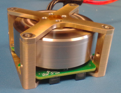

In my work on the Dellingr project, I have been tasked with getting the reaction wheels working. The reaction wheels are from Sinclair Interplanetary, and are used for attitude control (pictured right... the Sinclair website has much prettier photos). The first part of the task was relatively simple: communicate with the wheel over I^2^C. The second part is out of my league: model the wheel so that the person writing the control software can plug it into their system.

But that is the great thing about CubeSats: the teams are so small that you end up working on lots of different subsystems, even those outside of your comfort zone. You end up learning a lot out of necessity.

In flight, the satellite will be able to control the direction in which it is pointing (attitude control) by applying torques to its three reaction wheels. This torque results in the wheel spinning faster (or slower), as well as an opposite and equal reaction: the satellite will spin in the opposite direction. With three reaction wheels, one for each axis, the satellite will be able to orient itself as desired.

Reaction wheels are used on a large number of satellites, since they enable a high degree of pointing accuracy and do not need any fuel. For an amazing example, take a look at Kepler, the exo-planet hunting satellite. Unfortunately reaction wheels are not known for their long mission life, so satellites often include a fourth for redundancy. After Kepler's 2nd wheel failure (this was well after the primary mission was accomplished), an ingenuous solution was devised: Second Light. It's a bit of a tangent, but gives a good idea of the challenges facing satellites.

Grey-Box

So, I need a model of the reaction wheel. A function which gives me the change in acceleration based on current and speed. My first attempt, in following any number of tutorials available, was to start from the ground up. The "white-box" approach.

There is something about sitting down at a problem and starting with a fundamental law like F=MxA and building up from there. Unfortunately, the wheel is much to complicated for such analysis, with two levels of controllers already in place.

Another option is to treat the system like a "black-box": nothing of the internals is known, and one must observe the behavior through experiments. This is simpler, but the choice of test parameters becomes paramount as the results will only be applicable to those parameters. This can also be of use, for example one can avoid saturating the wheel which may be difficult to analyse.

My final approach (as advised by several people) was to treat the system mainly as an unknown, except for a few assumptions about drag. Thus the "grey-box." I assume that when the power is turned off, there is some forces acting on the wheel that will cause it to come to a stop, which seems reasonable.

Coasting

To isolate the drag, we can perform a "coast-down" test. The wheel is spun up to a high speed, and then power is turned off. We can then measure the speed at set intervals as the wheel comes to a rest. For good measure this is repeated several times.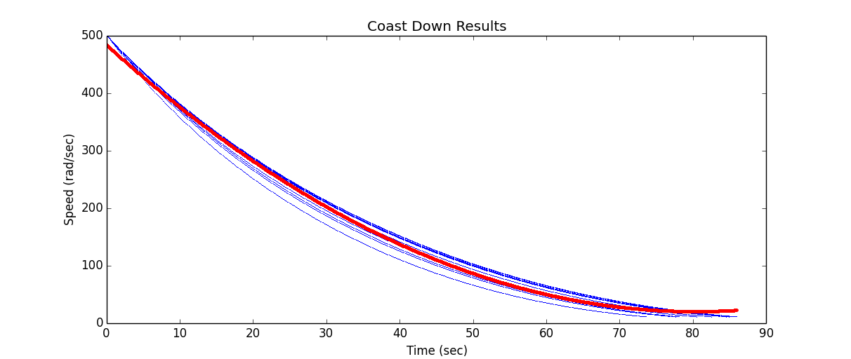

Here we see the speed of the wheel versus time for ten test runs. Also included is a curve fitting the data (in red). This curve is a 2^nd order polynomial: 0.07173x² - 11.53x + 483.9, where x is the time and the result is the speed.

The curve matches our data, but it is not actually what we are interested in. What we want is a curve relating the speed to the acceleration. So first we need to convert the speed data to acceleration, and then fit a curve to the new data.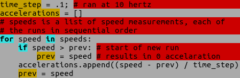

Convert from speed to acceleration.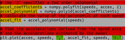

Fit a polynomial using NumPy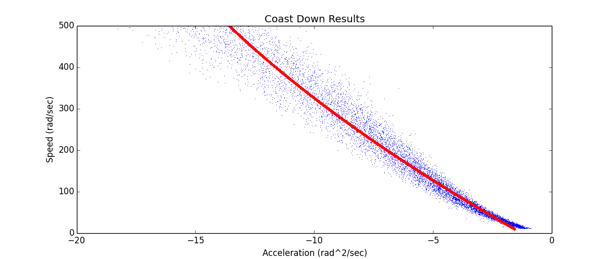

The curve shown here is: .00001258x² - 0.03095x - 1.262 A line also appears to fit well, which is not surprising due to the tiny 2^nd order coefficient above: -0.02539x - 1.602

Link to all code

Close Enough

The lower order polynomial we choose, the better the performance but the worse the fit. For the speed versus acceleration data, both a simple line (1^st order) and a quadratic function (2^nd order). So the question is, can we get away with using the simpler model?

A standard way of evaluating the fit of a model to data is to calculate the Coefficient of Determination, also called R².

Attach:r_squared_code_snip.png Δ

Finish this section

Speed Up

Now that we have an approximation for drag, we can move on to driving the wheel by adding current. For this we can run a whole new set of tests, this time commanding the wheel to maintain a set current. Again, we are interested in the acceleration.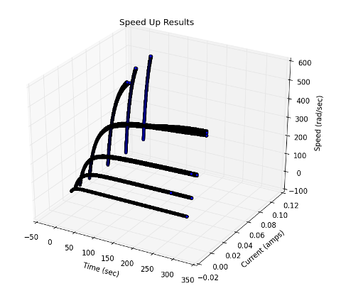

Speed Vs Time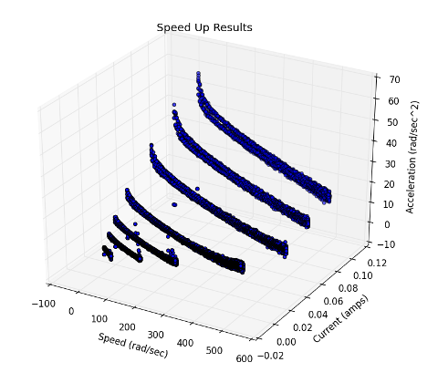

Acceleration resulting from Speed and Current

This time, however, we have two variables: the acceleration is a result of the speed and current. So instead of fitting a line or curve, we are fitting a surface.

Attach:speed_up_curve_fit.jpeg Δ

In Vacuum

This is all well and good, but the wheel is actually going to be used is space, which means that our atmospheric drag should not be a factor. Luckily we have a vacuum chamber here, so the tests can all be re-run in vacuum.

The expected (hoped for) result is that the drag function will change (no drag from air) and the acceleration due to current will remain the same.

Attach something here?

In Vacuum at 0°C

Especially since the satellite is so small, the wheel will likely see a range of temperatures. Somewhere in the range of -10°C to 50°C every orbit. The wheel's internal temperature during earlier test runs was usually around 30°C, so it would be nice to see how it runs near the lower end of the spectrum.

I swear this is the last round of tests. I hope.

Sanity

Do the fits from vacuum and atmosphere match when the estimated drag has been removed?

Conclusion

Don't hire a computer scientist to do system identification?